Intro to Probability Distributions

Probability is a branch of mathematics concerned with measuring the likelihood of events. In statistics, probability is used to make inferences about populations based on samples of data. Probability is typically represented as a number between 0 and 1, with 0 indicating an impossible event and 1 indicating a certain event.

We know that if we flip a coin the probability of getting heads or tails is .5. Rolling a single die, we know the probability is 1/6 for each side. As a reminder, we know that all these are independent of one another. Just because we flip three heads in a row, does not mean that we have a greater likelihood of flipping a tails on the next flip

If we take all of those probabilities of an event occurring (for flipping a coin there are 2 events: flipping a heads or flipping a tails) and plotted them, we would have a probability distribution. These probability distributions are a critical part of understanding statistics.

Probability distributions can operate on discrete data, where measured values cannot be subdivided (such as number of individuals), or on continuous data, where values can be subdivided or measured with greater accuracy (such as length).

Lets show some examples. On a probability distribution the y-axis indicates the probability density, or how probable a given event is, and the x-axis corresponds to some outcome.

If we had a probability distribution for rolling a single die we would have a discrete distribution, as you can only roll a 1, 2, 3, 4, 5, or 6, and it would be uniform as each value has equal probability of being rolled.

 But let’s show a more biological example.

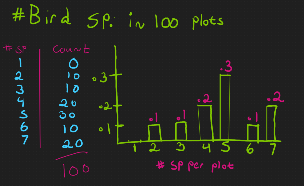
Below is a figure displaying the # of bird species detected in 100 different plots. Some plots had 2 species while others had 3 species or 4 species and so on and so forth. We can then create a probability distribution that shows the proportional amount of times that each # of species was detected. In the example below, 30 out of 100 plots had 5 species, so it would have a proportional frequency of .3. 

Since you can’t have half a species, this distribution is considered discrete. From this distribution, we can easily calculate the probability of detecting X number of species in a plot. For example, we have a probability of .3 (30%) for a plot to have 5 bird species. This is the same as its relative frequency!

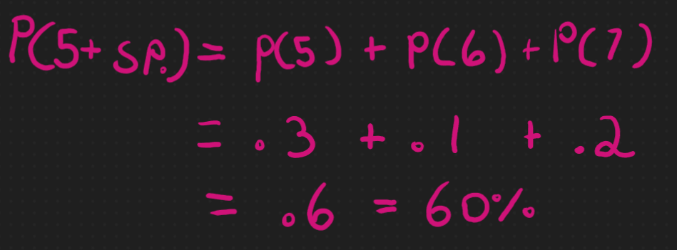
But we are not limited to single values! We can ask “What is the probability of a plot having 5 or more bird species?”

We can actually sum the probabilities of having 5, 6, and 7 bird species together and come up with .6 (60%)!

Naturally, this same concept applies to continuous probability distributions. Let’s say you measure the peak activity time of all those bird species and utilize time as a continuous variable. Time is continuous here because you can always subdivide it into smaller and smaller units. As another example, if we were measuring length we could measure in terms of meters, centimeters, millimeters, decimeters and so an so forth. With continuous data we can always subdivide or measure at greater accuracy.

Here our peak time was found to be 0600 (6am) and we expect time to peak activity to slowly ramp up, before slowly ramping back downwards. With continuous distributions, it’s often not useful to take the probability of a single point, because there are far too many subdivided units within the distribution. If we ask “What is the probability of peak activity being at precisely 0600?” we will find a very small probability. Who’s to say peak activity isn’t at 0601 (6:01 am), or 0600:01 (6 am and 1 second), or 0600:00:25 (6 am and 25 milliseconds)?

As such, we typically use ranges of data with probability distributions. We can ask “What is the probability of peak activity being between 0600 and 0800?” or “What is the probability of peak activity time occurring before 0700?”. In order to find those probabilities, we take the area under the curve! 

It may help to think of a continuous distribution as a discrete distribution but with an infinite number of values. If every single possible value between 0600 and 0800 was represented by its own bar, we could add each value’s probability together exactly the same as a discrete distribution. Of course, this is not easy to do by hand. Luckily, we have computer software to do that for us!