Intro to Functions

Intro to Functions

Functions are self contained bundles of code that provide some output when given an input. One example is sum(). The sum() function takes a vector of numeric values (input) and calculates the sum of all those values (output).

sum(c(1,2,34,6,5,4,2,83))

## [1] 137

There are many more functions that accomplish a wide variety of tasks. Any function in R uses arguments to accept some variable.

When we call a function, we include arguments which are separated by commas. To find the order of arguments in a function, you can check the documentation (use ?functionName). For these arguments, we can provide objects, a TRUE/FALSE value, or some text that instructs the function in some way.

We can explicitly specify which argument we want to use by using the name of the argument with an equal sign.

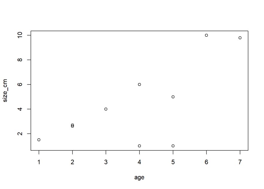
Lets showcase arguments, using the plot function. 

#lets first make some equal length vectors of data
age <- c(1,2,5,4,5,4,2,3,7,6)
size_cm <- c(1.5,2.6,1,1,5,6,2.7,4,9.8,10)
#then we can plot that data using the arguments x and y. 
# argument x relates to the data you place on the x axis
# argument y relates to the data you place on the y axis
plot(x = age, y = size_cm)

Arguments are described by each function in detail and placed in a particular order. For example, with plot() x is the first argument, while y is the second.

This order can be shuffled if we explicitly define each argument. For example, this chunk shows how to plot age and size_cm correctly in 3 different ways.

plot(age,size_cm) 
plot(x = age, y = size_cm)
plot(y = size_cm, x = age)

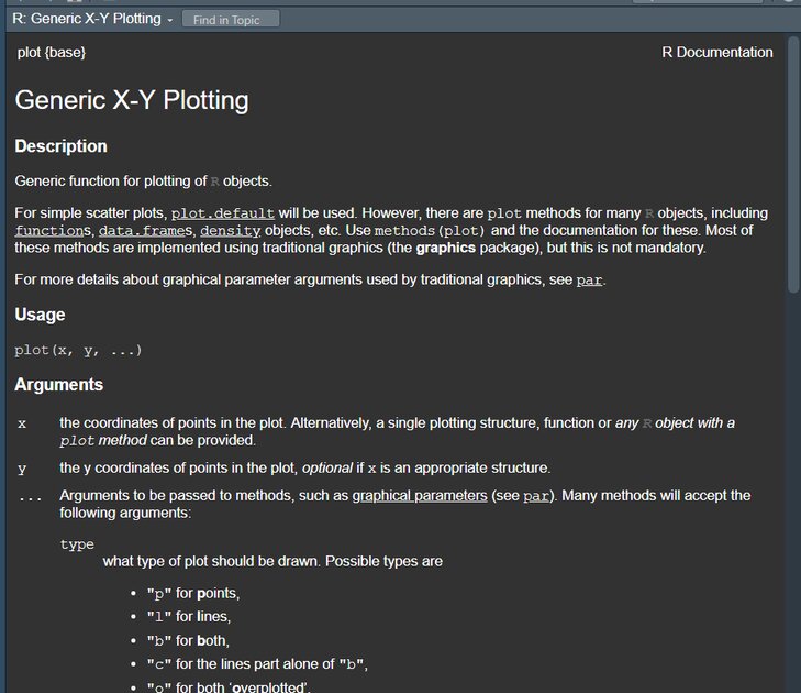
Naturally, functions can take many different arguments. To understand more about a function and what arguments it takes, we can place a question mark in front of the function to access its help documentation.

An example of the help window is shown below. If you run this on your own device, it will appear in the bottom right pane.

?plot

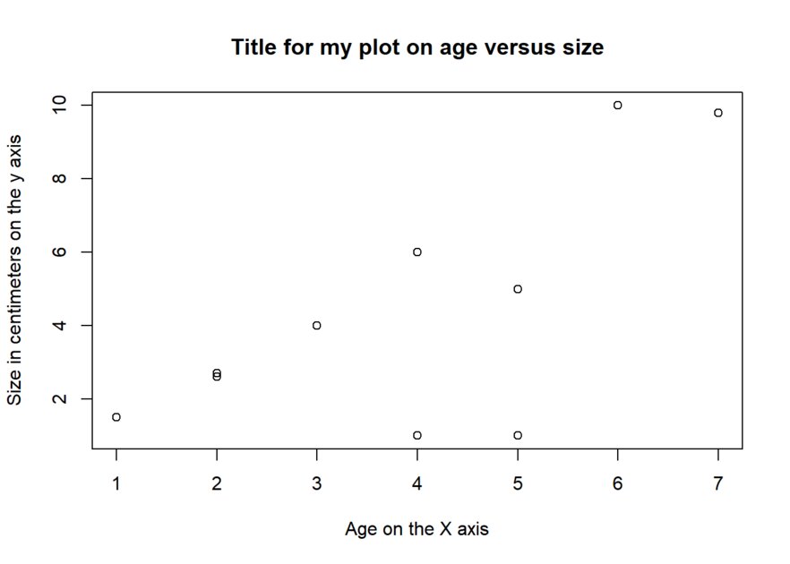
We can also make our functions easier to read by splitting them between multiple rows at each argument. To do so, you need to ensure that the function parentheses still contain all the arguments, and that each line is separated by a comma

#then we can plot that data using the arguments x and y. 
# x relates to the data you place on the x axis
# y relates to the data you place on the y axis
# xlab adds a label on the x axis
# ylab adds a label on the y axis
# main adds a title to the plot
plot(x = age, y = size_cm,
     xlab = "Age on the X axis",
     ylab = "Size in centimeters on the y axis",
     main = "Title for my plot on age versus size")

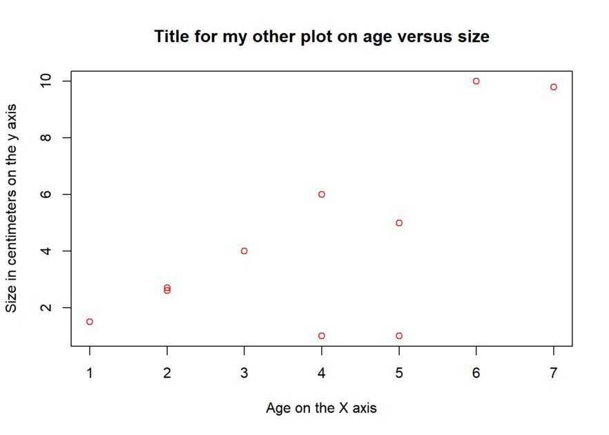
Again, if you are explicitly defining the arguments in your function, the order they appear does not matter.

#The following code will produce the same plot, even if the order of these arguments doesnt really make sense. I changed the point color to red in the second plot to make it clearer as to which plot is which. 
plot(xlab = "Age on the X axis",
     ylab = "Size in centimeters on the y axis",
     x = age,  main = "Title for my other plot on age versus size",
     y = size_cm, col = "red")

Functions are what we will mostly be working with in R. The beauty of R being an open source software, is that anyone can write their own functions and distribute them to other users through packages. Including you!